Getting Started: Isotropic Plate Example¶

This example walks through setting up a simple stress analysis for a square isotropic plate with a circular cutout in the center, subjected to uniaxial tension. In Panelyze, boundary condition inputs default to running loads (e.g., $lbf/in$), which is standard for thin-panel aerospace analysis.

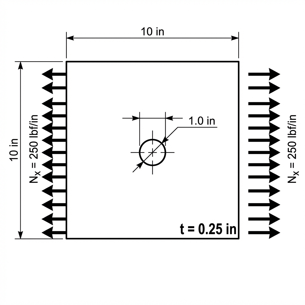
Problem Description¶

We will analyze a 10.0 in x 10.0 in square plate with a 1.0 in diameter hole (radius $R = 0.5 \text{ in}$) at the center. The panel thickness is 0.25 in. The material is aluminum (isotropic), and we apply a 250 lbf/in running load to the horizontal edges (equivalent to 1,000 psi stress).

Free Body Diagram (FBD)¶

Free Body Diagram of Isotropic Plate with Hole

Simulation Workflow¶

The following chart outlines the process for setting up and solving a problem in Panl:

        graph TD
    A[Material Definition] --> B[Geometry Creation]
    B --> C[Boundary Discretization]
    C --> D[Matrix Assembly]
    D --> E[Apply BCs & Constraints]
    E --> F[Solve Unknowns]
    F --> G[Extract Results]

Step-by-Step Implementation¶

1. Define the Material¶

For an isotropic material, we set $E_1 = E_2$ and calculate $G_{12}$ from $E$ and $\nu$. We specify a thickness of 0.25 in.

import numpy as np
from panl.analysis.material import OrthotropicMaterial

E = 10.0e6  # psi (Aluminum)
nu = 0.33
G = E / (2 * (1 + nu))

# Use pseudo-isotropic modulus to avoid Lechenitskii singularity
mat = OrthotropicMaterial(e1=E, e2=E*1.001, nu12=nu, g12=G, thickness=0.25)

2. Create Geometry and Mesh¶

Define the panel dimensions and add a circular cutout.

from panl.analysis.geometry import PanelGeometry, CircularCutout

W, H = 10.0, 10.0
radius = 0.5
geom = PanelGeometry(W, H)
geom.add_cutout(CircularCutout(x_center=W/2, y_center=H/2, radius=radius))

# Discretize the boundary
n_side = 20
elements = geom.discretize(num_elements_per_side=n_side, num_elements_cutout=80)

3. Assemble and Solve¶

Using the BEMKernels and BEMSolver. By default, the solve method treats BC values as running loads ($lbf/in$).

from panl.analysis.kernels import BEMKernels
from panl.analysis.solver import BEMSolver

kernels = BEMKernels(mat)
solver = BEMSolver(kernels, geom)
solver.assemble()

# Define Boundary Conditions (BCs)
num_dofs = 2 * len(elements)
bc_type = np.zeros(num_dofs, dtype=int)  # 0 = Traction (Running Load) given
bc_value = np.zeros(num_dofs)

# 1. Apply Running Load BCs (250 lbf/in Tension)
q_applied = 250.0
for i, el in enumerate(elements):
    if np.isclose(el.center[0], 0.0): # Left Edge
        bc_value[2*i] = -q_applied
    elif np.isclose(el.center[0], W): # Right Edge
        bc_value[2*i] = q_applied

# 2. Apply Displacement BCs (Corner Constraints)
bc_type[0:2] = 1
bc_value[0:2] = 0.0

k_br = n_side - 1
bc_type[2*k_br + 1] = 1
bc_value[2*k_br + 1] = 0.0

u, t = solver.solve(bc_type, bc_value)

4. Extract Results¶

Evaluate the stress ($psi$) and force resultants ($lbf/in$) at the stress concentration point.

# Point at theta=90 deg relative to hole center (r=0.51 in)
eval_pt = np.array([[W/2, H/2 + 0.51]])
stresses = solver.compute_stress(eval_pt, u, t)
resultants = solver.compute_resultants(eval_pt, u, t)

print(f"Sigma_xx at hole pole: {stresses[0, 0]:.1f} psi")
print(f"Nx at hole pole: {resultants[0, 0]:.1f} lbf/in")

Verification Results¶

The following code block is verified during documentation builds.

import numpy as np
from panl.analysis.material import OrthotropicMaterial
from panl.analysis.geometry import PanelGeometry, CircularCutout
from panl.analysis.kernels import BEMKernels
from panl.analysis.solver import BEMSolver
from panl.analysis import plot_results

E, nu = 10.0e6, 0.33
G = E / (2 * (1 + nu))
thickness = 0.25
mat = OrthotropicMaterial(e1=E, e2=E*1.001, nu12=nu, g12=G, thickness=thickness)

W, H = 10.0, 10.0
geom = PanelGeometry(W, H)
geom.add_cutout(CircularCutout(W/2, H/2, 0.5))

n_side = 20
elements = geom.discretize(num_elements_per_side=n_side, num_elements_cutout=80)

solver = BEMSolver(BEMKernels(mat), geom)
solver.assemble()

bc_type = np.zeros(2 * len(elements), dtype=int)
bc_value = np.zeros(2 * len(elements))

q_applied = 250.0
for i, el in enumerate(elements):
    if np.isclose(el.center[0], 0.0): bc_value[2*i] = -q_applied
    if np.isclose(el.center[0], W):   bc_value[2*i] = q_applied

bc_type[0:2] = 1
bc_value[0:2] = 0.0
bc_type[2*(n_side - 1) + 1] = 1
bc_value[2*(n_side - 1) + 1] = 0.0

u, t = solver.solve(bc_type, bc_value)

eval_pts = np.array([[W/2, H/2 + 0.51]])
stress = solver.compute_stress(eval_pts, u, t)

# Expect SCF ~2.94 based on stress
q_sigma = q_applied / thickness
scf = stress[0, 0] / q_sigma
print(f"Stress: {stress[0, 0]:.0f} psi")
print(f"SCF: {scf:.2f}")

# After solving the system
fig = plot_results(
   solver,
   u,
   t,
   deform_scale=100.0,
   title="Circular Cutout under X-Tension"
)
fig.show()

Stress: 2944 psi
SCF: 2.94